Methodology
- Background
- Previous Prediction Methods
- Method Used in Current Model
- Accuracy of Results Qualification
- References
Background
Galvanizing produces a zinc coating on the steel surface and is one of the most effective methods for corrosion protection of steel. This is attributed to the excellent corrosion resistance of zinc coatings, particularly in atmospheric environments. Galvanized steel is the most important application of zinc. Worldwide, the use of zinc for galvanizing results in an annual consumption of more than three million tons of zinc, constituting nearly one-half of the world zinc production [1].
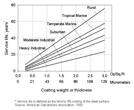
Figure 1
Corrosion rates for zinc, like other metals can vary by as much as two orders of magnitude in atmospheric environments depending on the specific environmental conditions. Therefore, it is important to know the specific corrosion rate in a given application environment in order to effectively use zinc coated steels in outdoor structures.
The most commonly used method, for corrosion life estimation of galvanized steels has been the use of generalized values (see Figure 1) for the different types of atmospheres [2]. However, although simple and convenient to use, this non-specific approach is no longer adequate to meet the demands of the market place. Today, designers and specifiers of galvanized steel increasingly ask information or performance certainty. Also, as products are becoming more application-specific, more relevant information on corrosion rates is required, generating the need for more accurate prediction methods.
Previous Prediction Methods
Numerous investigations have indicated that corrosion rates are strongly affected by certain factors, such as time of wetness, sulfur dioxide and chloride concentrations in the air. These findings form the basis for corrosion rate and lifetime prediction. Historically, there have been a number of methods developed to predict the life of galvanized steels in atmospheric environments. Each of these approaches is described briefly in the following.
-
Generalized Value Method
This method uses a generalized value to represent the corrosion rates in each typical environment. As shown in Figure 1, it provides simplified corrosion life data for six predetermined atmospheric environments. It can be easily seen that this method provides only a rough and non-specific estimation of product life since it uses only a few fixed values to account for the wide variation of real corrosion rates in one type of environment.
-
Geographic Mapping Method
In this method, corrosion rates of materials in a geographic area are determined and classified within a grid of sites to map the corrosivity of the area [5]. It recognizes the difficulty of using general corrosion rate prediction and attempts to estimate product service life based directly on field data from the service site in question. Thus, it is the most reliable method for estimation of product life. However, its usefulness is limited to the areas where such mapping is available and there are relatively few regions of the world that have been suitably mapped for this purpose.
-
ISOCORRAG
This is an environmental corrosivity classification system which was developed by the International Standard Organization (ISO) [6]. It divides atmospheric environments into five categories according to the values of time of wetness, sulfur dioxide and salt contents which have been correlated with the corrosion rates. It is a more accurate way of categorizing the atmospheric environments than the generalized value method and, thus, the estimated corrosion rate is more relevant to specific environmental conditions. However, it is still a rather approximate estimation, using only five ranges to account for two orders of magnitude in the variation of corrosion rates. In addition, since it accounts for the factors in a simple additive fashion, even the accuracy of the large categories themselves are questionable in some situations [7].
-
Regression Models
In this approach, mathematical functions are empirically formulated based on the statistical analysis of historical data with respect to the relevant factors. The following are three examples of such corrosion rate formulae.
- R = (a×SO2 + b×Cl + c)t (Ref. 8)
- R = a + b×SO2 + c×TOW + d×Cl (Ref. 9)
-
R = A×tn-1
where n = g + h×SO2(1 + i× T) + j×T
and A = a + b×Cl(1 + c×T + d× TOW) + e×SO2(1 + f×T) (Ref. 10,11)
in which R is corrosion rate, t is time, T is temperature, TOW is time of wetness, SO2 is sulfur dioxide level, Cl is chloride level, and a, b, c, d, e, f, g, h, i and j are constants.
While these models generally provide some useful correlation between corrosion rates and the factors for the data used in the regression analysis, a large uncertainty may be generated when they are used for prediction in environments which are not included in the regression analysis. This is mainly due to the fact that regression models use predetermined functions for a few factors, in a generally additive and linear fashion, while the real function for the effect of all the significant factors is essentially unknown. In addition, the data used in the development of the regression models are generally limited to a small number of atmospheres so that each model is limited in its applicability to of the diversity of atmospheric environments in the world.
Method Used in Current Model
The prediction models used in the current Zinc Coating Life Predictor were developed using neural network technology together with statistic methods. A commercial neural network software, NearoShell® 2, was used for the development of the predictions models [12].
- Neural Network Technology
Neural network technology mimics the brain's own problem solving process [12]. Just as humans apply knowledge gained from past experience to new problems or situations, a neural network takes previously solved examples to build a system of "neurons" that makes new decisions, classifications, and forecasts.
Neural networks look for patterns in training sets of data, learn these patterns, and develop the ability to correctly classify new patterns or to make forecasts and predictions. Neural networks excel at problem diagnosis, decision making, prediction, and other classifying problems where pattern recognition is important and precise computational answers are not required.
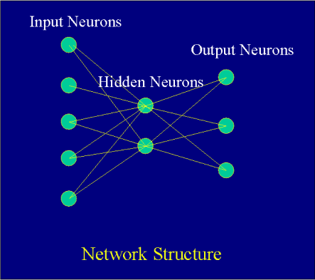
Figure 4The basic building block of neural network technology is the simulated neuron (depicted in Figure 4 as a circle). Independent neurons are of little use, however, unless they are interconnected in a network of neurons. The network processes a number of inputs from the outside world to produce an output, the network's classifications or predictions. The neurons are connected by "weights", (depicted as lines) which are applied to values passed from one neuron to the next.
Neurons are also grouped into layers by their connection to the outside world. For example, if a neuron receives data from outside of the network, it is considered to be in the input layer. If a neuron contains the network's predictions or classifications, it is in the output layer. Neurons in between the input and output layers are in the hidden layer(s).
A typical neural network is a Backpropagation network which usually has three layers of neurons. Input values in the first layer are weighted and passed to the second (hidden) layer. Neurons in the hidden layer "fire" or produce outputs that are based upon the sum of weighted values passed to them. The hidden layer passes values to the output layer in the same fashion, and the output layer produces the desired results (predictions or classifications).
The network "learns" by adjusting the interconnection weights between layers. The answers the network is producing are repeatedly compared with the correct answers, and each time the connecting weights are adjusted slightly in the direction of the correct answers. Eventually, if the problem can be learned, a stable set of weights adaptively evolves and will produce good answers for all of the sample decisions or predictions. The real power of neural networks is evident when the trained network is able to produce good results for data which the network has never "seen" before.
Accuracy of Results
-
Certainty of Prediction
Statistically, the average error of prediction using the models in this software is 36% ±13 at 95% confidence level. This is based on validation testing for more than 40 sets of field data representing different geographic locations which were not included in the training of the neural network models. Possible sources of error include the following:
- One important source of error is related to the inclusion of only a limited number of factors in the prediction model. Only six parameters were included: rain, RH, temperature, chloride concentration, sulfur concentration and time of exposure. In reality, many environmental, materials, and structural factors such as wind direction, frequency drying, minor alloying composition, and surface orientation etc. may also affect corrosion rate but were not used because these parameters were found to be less significant than those listed above and generally not monitored in normal atmospheric testing. There are very limited amounts of field data available for parameters other than the six selected also, this model.
- A major source of error lies in the difference between the nature of the corrosion rate determined experimentally and the rate calculated. Each piece of field data is a time-averaged value determined by the instantaneous environmental parameters. On the other hand, the calculated rate is obtained using the annual average of the environmental parameters.
- A third source of error is related to the uneven representation and to the inconsistency of the field data available for the model development. The data on the corrosion rates of zinc in various locations in the world were obtained from investigations conducted by a large number of researchers in different countries and in different time periods. The material conditions and testing procedures in these investigations were likely significantly different from each other.
The average error of about 36% for the predicted corrosion rate values is an indication of the variance caused by the three error sources mentioned above. Nevertheless, the corrosion rate generated by the prediction model, which considers the six parameters, accounts for 64% of the variance of the zinc atmospheric corrosion system.
-
Comparison with ISO Method
The International Standard Organization, ISO, in 1993 published a standard, ISO 9223, on "Corrosion of metals and alloys - corrosivity of atmospheres - classification" [6]. It classifies atmospheric environments into five rate ranges according to three environmental parameters: time of wetness, sulfur dioxide and salt contents. As illustrated in Figure 5 the combination of the three environmental parameters determines the specific corrosion rate. The current Zinc Coating Life Predictor model differs from the ISO model in the following ways:
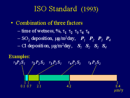
Figure 5- It provides a specific value while the ISO method gives a range of values for given ranges of conditions.
- It is a continuous function of the factors while the ISO method uses 4 or 5 broad ranges of the values for the factors.
- It uses original climate parameters, (i.e. temperature and relative humidity) instead of just the time of wetness which has to be deduced from temperature and relative humidity data. In practical situations, it is much easier to obtain annual avenge temperature and relative humidity than time of wetness which is not a common parameter provided by a weather station.
- It considers the specific effect of rain while the ISO method does not. It thus responds more realistically to the situations where rain is a significant factor.
References
- International Lead Zinc Study Group, Zinc and Lead Statistics, London, UK, 1996.
- American Galvanisers Association, "Galvanizing for Corrosion Protection -- A Special Guide", 1990.
- X.G. Zhang, "Corrosion and Electrochemistry of Zinc", Plenum, New York, 1996.
- Cominco Ltd., unpublished data.
- G.A. King, "Corrosivity Mapping - A Novel Tool for Materials Selection and Asset Management", Materials Performance, January, p. 6, 1995.
- International Standard, "Corrosion of Metals and Alloys -- Corrosivity of Atmospheres -- Classification", ISO 9223, 1992.
- G.A. King, "Some Apparent Limitations in Using the ISO Atmospheric Corrosivity Categories", Corrosion and Materials, Vol. 23, February, p. 8, 1998.
- V. Kucera, S. Haagenrud, L. Atteraas and J. Gullman, "Corrosion of Steel and Zinc in Scandinavia With Respect to the Classification of the Corrosivity of Atmospheres", in Degradation of Metals in the Atmosphere, eds. S.W. Dean and T.S. Lee, ASTM STP 965, p. 264, 1982.
- Knotkova, D., Boschek, P. and Kreislova, K., "Results of ISO CORRAG Program: Processing of One-Year Data in Respect to Corrosivity Classification", ASTM STP 1239, W.W. Kirk and H.H. Lawson, ASTM Philadelphia, p. 38, 1995.
- Feliu, S., Morcillo, M. and Feliu, S., "The Prediction of Atmospheric Corrosion from Meteorological and Pollution Parameters - I. Annual Corrosion", Corrosion Science, Vol. 34, p. 403, 1993.
- Feliu, S., Morcillo, M. and Feliu, S. Jr, "The Prediction of Atmospheric Corrosion from Meteorological and Pollution Parameters - II. Long-Term Forecasts", Corrosion Science, Vol. 34, p. 415, 1993.
- NeuralShell 2, Ward System Group, Inc.Fourth Edition, Frederick, MD,1996.